Map reduce with examples

MapReduce

Problem: Can’t use a single computer to process the data (take too long to process data).

Solution: Use a group of interconnected computers (processor, and memory independent).

Problem: Conventional algorithms are not designed around memory independence.

Solution: MapReduce

Definition. MapReduce is a programming paradigm model of using parallel, distributed algorithims to process or generate data sets. MapRedeuce is composed of two main functions:

Map(k,v): Filters and sorts data.

Reduce(k,v): Aggregates data according to keys (k).

MapReduce Phases

MapReduce is broken down into several steps:

Record Reader
Map
Combiner (Optional)
Partitioner
Shuffle and Sort
Reduce
Output Format

Record Reader

Record Reader splits input into fixed-size pieces for each mapper.

The key is positional information (the number of bytes from start of file) and the value is the chunk of data composing a single record.

alt text

In hadoop, each map task’s is an input split which is usually simply a HDFS block
Hadoop tries scheduling map tasks on nodes where that block is stored (data locality)
If a file is broken mid-record in a block, hadoop requests the additional information from the next block in the series

Map

Map User defined function outputing intermediate key-value pairs alt text

key ( $k_{2}$ ): Later, MapReduce will group and possibly aggregate data according to these keys, choosing the right keys is here is important for a good MapReduce job.

value ( $v_{2}$ ): The data to be grouped according to it’s keys.

Combiner (Optional)

Combiner UDF that aggregates data according to intermediate keys on a mapper node alt text

This can usually reduce the amount of data to be sent over the network increasing efficiency

$\left.\begin{array}{r} \left(\mbox{"hello world"},1\right)\\ \left(\mbox{"hello world"},1\right)\\ \left(\mbox{"hello world"},1\right) \end{array}\right\} \overset{\mbox{combiner}}{\longrightarrow}\left(\mbox{"hello world"},3\right)$

Combiner should be written with the idea that it is executed over most but not all map tasks. ie. $\left(k_{2},v_{2}\right)\mapsto\left(k_{2},v_{2}\right)$
Usually very similar or the same code as the reduce method.

Partitioner

Partitioner Sends intermediate key-value pairs (k,v) to reducer by $\mbox{Reducer}=\mbox{hash}\left(\mbox{k}\right)\pmod{R}$
alt text

will usually result in a roughly balanced load accross the reducers while ensuring that all key-value pairs are grouped by their key on a single reducer.
A balancer system is in place for the cases when the key-values are too unevenly distributed.
In hadoop, the intermediate keys ( $k_{2},v_{2}$ ) are written to the local harddrive and grouped by which reduce they will be sent to and their key.

Shuffle and Sort

Shuffle and Sort On reducer node, sorts by key to help group equivalent keys alt text

Reduce

Reduce User Defined Function that aggregates data (v) according to keys (k) to send key-value pairs to output alt text

Output Format

Output Format Translates final key-value pairs to file format (tab-seperated by default). alt text

MapReduce Example: Word Count

alt text
Image Source: Xiaochong Zhang’s Blog

DAG Models

A more flexible form of MapReduce is used by Spark using Directed Acyclic Graphs (DAG). alt text

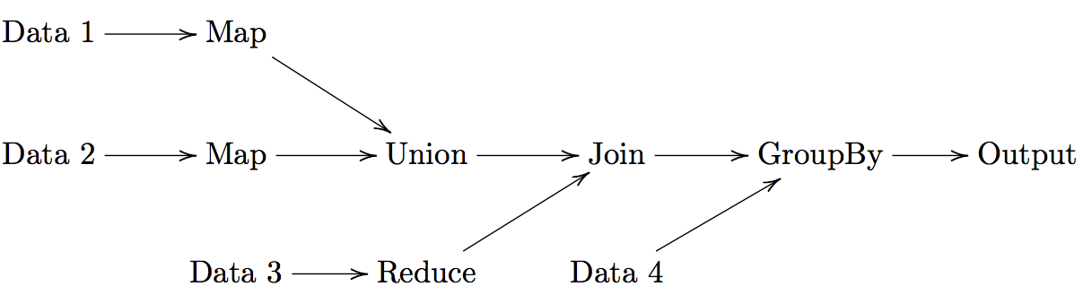
For a set of operations:

Create a DAG for operations
Divide DAG into tasks
Assign tasks to nodes

MapReduce Programming Models

Looking for parameter(s) ( $\theta$ ) of a model (mean, parameters of regression, etc.)

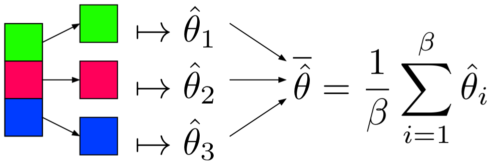
Partition and Model:
1. Partition data,
2. Apply unbiased estimator,
3. Average results.
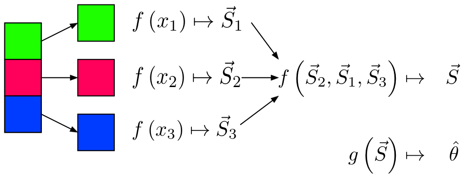
Sketching / Sufficient Statistics:
1. Partition data,
2. Reduce dimensionality of data applicable to model (sufficient statistic or sketch),
3. Construct model from sufficient statistic / sketch.

Partition and Model

alt text

Notes

$\overline{\hat{\theta}}$ is as efficient as $\hat{\theta}$ with the whole dataset when: 1. $\hat{\theta}\sim N\left(\theta,\sigma^{2}\right)$ 2. x is IID and 3. x is equally partitioned

Can use algorithms already in R, Python to get $\hat{\theta}_i$
$\overline{\hat{\theta}}\sim N\left(\theta,\frac{\sigma_{\hat{\theta}}^{2}}{\beta}\right)$ by Central Limit Theorem

Restrictions

Values must be IID (i.e. not sorted, etc.)
Model must produce an unbiased estimator of $\theta$ , denoted $\hat{\theta}$
$\sigma_{\hat{\theta}}^{2}<\infty$

Sketching / Sufficient Statistics

Streaming (Online) Algorithm: An algorithm in which the input is processed item by item. Due to limited memory and processing time, the algorithm produces a summary or “sketch” of the data.

Sufficient Statistic: A statistic with respect to a model and parameter $\theta$ , such that no other statistic from the sample will provide additional information.

Sketching / Sufficient Statistics programming model aims to break down the algorithm into sketches which is then passed off into the next phase of the algorithm.

alt text

Notes

Not all algorithms can be broken down this way.

Restrictions

All sketches must be communicative and associative
For each item to be processed, the order of operations must not matter

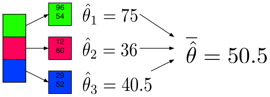
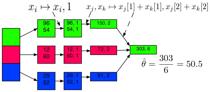
Example: Mean

Partition and Model

$\begin{aligned}\hat{\theta}=\frac{1}{n}\sum_{i=1}^{n}x_{i} & & \overline{\hat{\theta}}=\frac{1}{\beta}\sum_{i=1}^{\beta}\hat{\theta}_{i}\end{aligned}$ alt text

Sufficient Statistic / Sketch

alt text

Example: Mean Code

from numpy.random import randint, chisquare
import numpy as np
X = sc.parallelize(randint(0, 101, 200000))
X_part = X.repartition(10).cache()

Example: Mean + Partition and Model

def mean_part(interator):
    x = 0
    n = 0
    for i in interator:
        x+=i
        n+=1
    avg = x / float(n)
    return [[avg, n]]
model_mean_part = X_part.mapPartitions(mean_part)  \
    .collect()


model_mean_part



[[50.336245888157897, 19456],
 [50.215136718750003, 20480],
 [50.007421874999999, 20480],
 [50.135214401294498, 19776],
 [50.141858552631582, 19456],
 [50.08115748355263, 19456],
 [50.2578125, 20480],
 [50.243945312500003, 20480],
 [49.786543996710527, 19456],
 [50.072363281249999, 20480]]

Example: Mean + Partition and Model

The partitions are not equally sized, thus we’ll use a weighted average.

    def     (theta):
        total = 0
        weighted_avg = 0
        for i in xrange(len(theta)):
            weighted_avg += theta[i][0] * theta[i][1]
            total+= theta[i][1]
        theta_bar = weighted_avg / total
        return theta_bar
    print("Mean via Partition and Model:")
    weighted_avg(model_mean_part)

    Mean via Partition and Model:

    50.128590000000003

Example: Mean + Sufficient Statistics / Sketching

    sketch_mean = X_part.map(lambda num: (num, 1)) \
        .reduce(lambda x, y: (x[0]+y[0], x[1]+y[1]) ) 
    x_bar_sketch = sketch_mean[0] / float(sketch_mean[1])
    print("Mean via Sketching:")
    x_bar_sketch

    Mean via Sketching:





    50.128590000000003

Example: Variance

$\begin{aligned}\mbox{Sample Var}=\hat{\theta} & =\frac{1}{n-1}\sum_{i=1}^{n}\left(x_{i}-\overline{x}\right)^{2}\\ & =\frac{1}{n-1}\left[\sum_{i=1}^{n}x_{i}^{2}-n\times\left(\overline{x}\right)^{2}\right] \end{aligned}$

$\begin{aligned}\mbox{Sufficient Stat}=\sum_{i=1}^{N}x_{i}^{2}, & & \sum_{i=1}^{N}x_{i}, & & N\end{aligned}$

Example: Variance + Partition and Model

    def var_part(interator):
        x = 0
        x2 = 0
        n = 0
        for i in interator:
            x += i
            x2 += i **2
            n += 1
        avg = x / float(n)
        var = (x2 + n * avg ** 2) / (n-1)
        return [[var, n]]
    var_part_model = X_part.mapPartitions(var_part)   \
        .collect()
    print("Variance via Partitioning:")
    print(weighted_avg(var_part_model))

    Variance via Partitioning:
    851.095985421

Example: Variance + Sufficient Statistics / Sketching

    sketch_var = X_part.map(lambda num: (num, num**2, 1)) \
        .reduce(lambda x, y: (x[0]+y[0], x[1]+y[1], x[2]+y[2]) ) 
    x_bar_4 = sketch_var[0] / float(sketch_var[2])
    N = sketch_var[2]
    print("Variance via Sketching:")
    (sketch_var[1] + N * x_bar_4 ** 2 ) / (N -1) 

    Variance via Sketching:





    851.07917000774989

Linear Regression

To understand the MapReduce framework, lets solve a familar problem of Linear Regression. For Hadoop/MapReduce to work we MUST figure out how to parallelize our code, in other words how to use the hadoop system to only need to make a subset of our calculations on a subset of our data.

Assumption: The value of p, the number of explanatory variables is small enough for R to easily handle i.e.
$n\gg p$

We know from linear regression, that our estimate of $\hat{\beta}$ :
$X^{T}X\hat{\beta}=X^{T}y$

$\left(X^{T}X\right)_{p\times p}$ and $\left(X^{T}y\right)_{p\times1}$ is small enough for R to solve for $\hat{\beta}$ , thus we only need $X^{T}X,X^{T}y$ to get $\hat{\beta}$ .

To break up this calculation we break our matrix X into submatricies $X_{i}$ :
$X=\begin{bmatrix}X_{1}\\ X_{2}\\ X_{3}\\ \vdots\\ X_{n} \end{bmatrix} y=\begin{bmatrix}y_{1}\\ y_{2}\\ y_{3}\\ \vdots\\ y_{n} \end{bmatrix}$

$X^{T}X = \begin{bmatrix}X_{1}^{T} & X_{2}^{T} & X_{3}^{T} & \cdots & X_{n}^{T}\end{bmatrix}\begin{bmatrix}X_{1}\\ X_{2}\\ X_{3}\\ \vdots\\ X_{n} \end{bmatrix} \implies$ $X^{T}X = \begin{bmatrix}X_{1}^{T}X_{1}+ & X_{2}^{T}X_{2}+ & X_{3}^{T}X_{3}+ & \cdots & +X_{n}^{T}X_{n}\end{bmatrix}$ $X^{T}y=\begin{bmatrix}X_{1}^{T} & X_{2}^{T} & X_{3}^{T} & \cdots & X_{n}^{T}\end{bmatrix}\begin{bmatrix}y_{1}\\ y_{2}\\ y_{3}\\ \vdots\\ y_{n} \end{bmatrix}\implies$ $X^{T}y=\begin{bmatrix}X_{1}^{T}y_{1}+ & X_{2}^{T}y_{2}+ & X_{3}^{T}y_{3}+ & \cdots & +X_{n}^{T}y_{n}\end{bmatrix}$

Sys.setenv("HADOOP_PREFIX"="/usr/local/hadoop/2.6.0")
Sys.setenv("HADOOP_CMD"="/usr/local/hadoop/2.6.0/bin/hadoop")
Sys.setenv("HADOOP_STREAMING"=
    "/usr/local/hadoop/2.6.0/share/hadoop/tools/lib/hadoop-streaming-2.6.0.jar")
library(rmr2)
library(data.table)
# Setup variables 
p = 10 
num.obs = 200
beta.true = 1:(p+1) 
X = cbind(rep(1,num.obs), matrix(rnorm(num.obs * p), 
    ncol = p))
y = X %*% beta.true + rnorm(num.obs) 
X.index = to.dfs(cbind(y, X)) 
rm(X, y, num.obs, p)

map.XtX = function(., Xi) {
    Xi = Xi[,-1] #Get rid of y values in Xi
    keyval(1, list(t(Xi) %*% Xi)) 
}
map.Xty = function(., Xi) {
    yi = Xi[,1] # Retrieve the y values
    Xi = Xi[,-1] #Get rid of y values in Xi
    keyval(1, list(t(Xi) %*% yi)) 
}
Sum = function(., YY) {
    keyval(1, list(Reduce('+', YY))) 
}


Sys.setenv("HADOOP_PREFIX"="/usr/local/hadoop/2.6.0")
Sys.setenv("HADOOP_CMD"="/usr/local/hadoop/2.6.0/bin/hadoop")
Sys.setenv("HADOOP_STREAMING"=
    "/usr/local/hadoop/2.6.0/share/hadoop/tools/lib/hadoop-streaming-2.6.0.jar")
library(rmr2)
library(data.table)
#Setup variables 
p = 10 
num.obs = 200
beta.true = 1:(p+1) 
X = cbind(rep(1,num.obs), matrix(rnorm(num.obs * p), 
    ncol = p))
y = X %*% beta.true + rnorm(num.obs) 
X.index = to.dfs(cbind(y, X)) 
rm(X, y, num.obs, p) 
##########################
map.XtX = function(., Xi) {
    Xi = Xi[,-1] #Get rid of y values in Xi
    keyval(1, list(t(Xi) %*% Xi)) 
}
map.Xty = function(., Xi) {
    yi = Xi[,1] # Retrieve the y values
    Xi = Xi[,-1] #Get rid of y values in Xi
    keyval(1, list(t(Xi) %*% yi)) 
}
Sum = function(., YY) {
    keyval(1, list(Reduce('+', YY))) 
}

The reason we are returning a list in the map function is because otherwise Reduce will only return a some of the elements of the matricies.

List prevents this by Reduce iterating though the elements of the list (the individual $X_{i}^{T}X_{i}$ matricies) and applying the binary function ‘+’ to each one.

List is used in the reduce function Sum because we will also use this as a combiner function and if we didn’t use a list we would have the same problem as above.

XtX = values(from.dfs(
    mapreduce(input = X.index,
    map = map.XtX,
    reduce = Sum,
    combine = TRUE)))[[1]]

Xty = values(from.dfs(
    mapreduce(
    input = X.index,
    map = map.Xty,
    reduce = Sum,
    combine = TRUE)))[[1]]
beta.hat = solve(XtX, Xty)
print(beta.hat)



XtX = values(from.dfs(
    mapreduce(input = X.index,
    map = map.XtX,
    reduce = Sum,
    combine = TRUE)))[[1]]

Xty = values(from.dfs(
    mapreduce(
    input = X.index,
    map = map.Xty,
    reduce = Sum,
    combine = TRUE)))[[1]]
beta.hat = solve(XtX, Xty)
print(beta.hat)


           [,1]
 [1,]  1.045835
 [2,]  1.980511
 [3,]  2.993829
 [4,]  4.011599
 [5,]  5.074755
 [6,]  6.008534
 [7,]  6.947164
 [8,]  8.024570
 [9,]  9.024757
[10,]  9.888609
[11,] 10.893023