How to install the python data science stack on linux or a remote linux server
Beginners Tutorial for How to Get Started Doing Data Science using Servers provided us with a background of why using servers are useful for data scientists and how setup and connect to a server using SSH. In this section we will learn how to install python and the common packages data scientists use with python which we call the PyDataScience Stack. We will also learn how to setup and use Jupyter get started with data analysis with python. This guide should also work for people using Mac and Linux on their local machines.
Anaconda Distribution
Continuum Analytics has developed a Anaconda Distribution which provides an installer and package management for the PyDataScience stack. While being free to use (even for commercial), it is not fully open sourced and their script (.sh file) includes precompiled binary code. Precompiled binary means that there was original source code used to generate the code you would be running. It is not recommended to blindly use precompiled code since the content of the original source code is unknown and can create security flaws on your server. For this reason is better to install packages on our own or using a fully open sourced package manager. If you choose to take the simpler (but not better route) of using the Anaconda distribution the specific instructions for your system (Linux, Mac and Windows) can be found on the downloads page
Installing the PyDataScience Framework Manually
First let us install some common utilities which are useful for using servers:
sudo apt-get -y install git curl vim tmux htop ranger
Next let us install python, python development and python-pip:
sudo apt-get -y install python2.7 python-dev python-pip
We an also install some optional python libraries which are popularly used:
sudo apt-get -y install python-serial python-setuptools python-smbus
Next we need to set up virtual environments for python. A Virtual Environment is a tool to keep the dependencies required by different projects in separate places, by creating virtual Python environments for them. It solves the “Project X depends on version 1.x but, Project Y needs version 4.x” dilemma, and keeps your global site-packages directory clean and manageable. For example, you can work on a data science project which requires Django 1.3 while also maintaining a project which requires Django 1.0.
Let us get started by installing virtualenv using pip
pip install virtualenv
If that command gave you an error, then it might be necessary to run all pip commands as super user (sudo pip install virtualenv) instead
Now lets create a folder in the home directory (~/) which will contain the Python executable files, and a copy of the pip library which you can use to install other packages. The name of the virtual environment (in this case, it is data-science) can be anything; omitting the name will place the files in the current directory instead.
  cd ~/
  mkdir venv
  pushd venv
  virtualenv data-science
  popd
Now let us activate our virtual environment.
source ~/venv/data-science/bin/activate
The name of the current virtual environment will now appear on the left of the prompt (e.g. (venv)Your-Computer:your_project UserName$) to let you know that it’s active. From now on, any package that you install using pip will be placed in the venv folder, isolated from the global Python installation. This means that When the virtual environment is activated, when anything is installed using pip, it is installed in the virtual environment, not in your system’s python. This means you can have different version of libraries installed and if an installation breaks, you can simply delete the corresponding venv folder (data-science in this case) and start over without damaging the global Python installation.
If you want to deactivate the virtual environment, it is as simple as using the deactivate command:
deactivate
Installing the Required Python Packages
If the virtual environment is not active, we can activate it again:
source ~/venv/data-science/bin/activate
Next let us upgrade our python setup tools and install compilation requirements in python:
  pip install --upgrade setuptools
  pip install virtualenvwrapper
  pip install cython
  pip install nose
Now that we have all of the requirements, let us begin by installing the SciPy stack
sudo apt-get -y install python-numpy python-scipy python-matplotlib ipython ipython-notebook python-pandas python-sympy python-nose
In the future you might also want to add the NeuroDebian repository for extra SciPy packages but for now let us move onto installing Jupyter notebook:
pip install jupyter
Jupyer notebook (or “notebooks”) are documents produced by the Jupyter Notebook App which contain both computer code (e.g. python) and rich text elements (paragraph, equations, figures, links, etc…). Notebook documents are both human-readable documents containing the analysis description and the results (figures, tables, etc..) as well as executable documents which can be run to perform data analysis.
Since some packages require matplotlib, we If you are on a Mac or Linux, and pip install matplotlib did not work, you are probably missing the supporting packages zlib, freetype2 and libpng. Let us install the requirements:
  sudo apt-get -y install libfreetype6-dev libpng12-dev libjs-mathjax fonts-mathjax libgcrypt11-dev libxft-dev

  pip install matplotlib
Next let us install the requirements for Seaborn, then install Seaborn itself, which is a very powerful statistical plotting library:
  sudo apt-get install libatlas-base-dev gfortran

  pip install Seaborn
A very complimentary powerful statistics library is statsmodels
pip install statsmodels
Let us now install one of the most powerful and commonly use machine learning library scitKit-learn
pip install scikit-learn
Now let us install some other python libraries which commonly used for data science:
pip install numexpr && pip install bottleneck && pip install pandas && pip install SQLAlchemy && pip install pyzmq && pip install jinja2 && pip install tornado
Next let us install two powerful packages for text processing: natural language toolkit and gensim: topic modelling for humans
  pip install nltk
  pip install gensim
We have now installed the most popular python libraries used for data science. There are many more packages which can be installed if necessary, but we have installed enough to get started. If you would prefer to use a dark theme for Jupyter notebook, you can follow the next subsection or you can move onto install R and Rstudio.
Jupyter Notebook Custom Themes (Optional)
This step is optional. Just like any other development environment, with Jupyter notebook, you can change the theme, color scheme and syntax highlighting. I personally prefer dark themes such as Oceans16, you can follow the following steps to choose a different theme.
pip install git+https://github.com/dunovank/jupyter-themes.git
We are going to install theme (-t) for ipython/jupyter version > 3.x (-J) with the toolbar (-T)
jupyter-theme -J -t oceans16 -T
Running Jupyter Notebook
Before we started running python code on our server, let us set some safety constraints to ensure that our code does not use all the CPU and memory resources. The first step is determining how much memory our system is using using the free command:
free
A sample output using the corn-syrup server from uWaterloo’s csclub is the following:
                total        used        free      shared  buff/cache   available
  Mem:       32947204      981132      201380      271260    31764692    31568324
  Swap:             0           0           0
Under the total column, the first number is the total memory available in kbytes. This means that there is 32947204 kbytes of RAM total or about 32 GB. It is generally suggested to not exceed 75% of memory to ensure the system does not hang or freeze, but you are free to set the limit to what ever you think is best. You can limit the memory using the following command
ulimit -m 20000000 ulimit -v 20000000
The -m is for the total memory, and the -v is for the virtual memory. In this example, the limit is set to 20000000 kbytes, which is equivalent to around 20GB.
You can see the limits by the following command:
ulimit -a
A sample output is the following:
  core file size          (blocks, -c) 0
  data seg size           (kbytes, -d) unlimited
  scheduling priority             (-e) 0
  file size               (blocks, -f) unlimited
  pending signals                 (-i) 13724
  max locked memory       (kbytes, -l) 64
  max memory size         (kbytes, -m) 20000000
  open files                      (-n) 1024
  pipe size            (512 bytes, -p) 8
  POSIX message queues     (bytes, -q) 819200
  real-time priority              (-r) 0
  stack size              (kbytes, -s) 8192
  cpu time               (seconds, -t) unlimited
  max user processes              (-u) 13724
  virtual memory          (kbytes, -v) 20000000
  file locks                      (-x) unlimited
Specifically we can see the memory limits by piping the output to the grep command and searching for the keyword memory:
ulimit -a | grep memory
The output is:
  max locked memory       (kbytes, -l) 64
  max memory size         (kbytes, -m) 20000000
  virtual memory          (kbytes, -v) 20000000
Next we can optionally run Jupyter using tmux so that is can run in the background, and not be terminated if you close terminal. Tmux is a very popular terminal multiplexer. What is a terminal multiplexer? It lets you switch easily between several programs in one terminal, detach them (they keep running in the background) and reattach them to a different terminal. This guide outlines how to install and use tmux, and this guide outlines how to configure tmux. We can how install tmux:
sudo apt-get update && sudo apt-get -y install tmux
You automatically login a tmux session to your default shell with your user account using the following command:
tmux
The default binding key to send commands to tmux is holding Ctrl and hitting b (Ctrl-b) You can detach by hitting
Ctrl-b d
You can reconnect by running the following command:
tmux attach
The two guides above outline more advanced things you can do with tmux such as creating multiple windows or panes. Once we have set the limits for the memory and are optionally running tmux, we can we can now run Jupyter notebook using the following command:
nice jupyter notebook
We use the nice command to lower the priority of the code running in Jupyter. This is important since if you are running very CPU intensive code, it will run at a lower priority. This means that not only will it not disrupt others using the server (if it is a shared resource) but it will also ensure that the intensive code has a lower priority than important system functions.
When you run Jupyter notebook, it runs on a specific port number. The first notebook you are running will run generally on port 8888 so you can simply navigate to localhost:8888 to connect to Jupyter notebook.
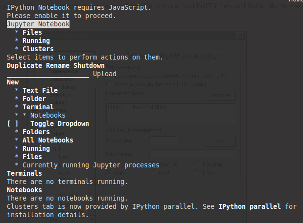
If you are running Jupyter on a a server without a web browser, it will still run but give you an error stating that Ipython notebook requires JavaScipt as shown below. This is expected since JavaScript is not necessary on a server without a web browser. You can type q and then enter on the keyboard and confirm by to closing w3m by hitting y and then enter which will remove the error message (and show you which port Jupyter is running on).
Since you are using tmux you can create a new pane or a new window and run the following command to monitor the system (and Jupyter):
htop
If you are not using tmux, you can open another ssh session to the server the run htop. Using htop, we can move around using the arrow keys, sort the processes by hitting F6, change the priority level using F8 and kill processes using F9. If you are using Mac and following these instructions on your local machine, you will need to run it using a super user (run sudo htop). In the next section We will learn how to connect to the web browser and use Jupyter as if it was running on your local computer.
Since Jupyter was run using nice, all python scripts run in Jupyter will appear in blue on htop indicating that they are running at a lower priority (compared to green and red).
Connecting to the server using SSH Tunneling
In this section we will learn how to connect to Jupyter notebook using SSH tunneling. While SSH tunneling might sound scary, the concept is very simple. Since Juptyer notebook is running on a specific port such as 8888, 8889 etc, SSH tunneling enables you to connect to the server’s port securely. Since we are used to running Jupyter notebook on a specific port number, we can create a secure tunnel which listens on the the server’s port (8888 for example) and securely forwards a port on our local computer on a specific port (8000 for example).
Mac or Linux
If using Linux of Mac, this can be done simply by running the following SSH command:
ssh -L 8888:localhost:8000 server_username@<server ip address>
You should change 8888 to the port which Jupyter notebook is running on, and optionally change port 8000 to one of your choosing (if 8000 is used by another process). Your server_username is your username on the server and the <server ip address> could be an actual IP address or a URL depending on who is providing your virtual machine. In the csclub example, the server_username is your csclub username (generally your quest ID) and the server ip would be for example corn-syrup.uwaterloo.ca. The command I would run if my username is andrew.andrade is:
ssh -L 8888:localhost:8000 andrew.andrade@corn-syrup.uwaterloo.ca
If no error shows up after running the ssh -L command and you tunneled the port to 8000 (for example), you can simply navigate to localhost:8000 in your favourite web browser to connect to Jupyer notebook running on the server!
Windows
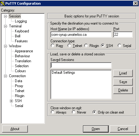
If you are using windows, you can also easily tunnel ssh using putty. As you may remember, you SSH into a server, you enter the server url into the host name as shown in the figure below (for connecting to corn-syrup from the uwaterloo csclub).
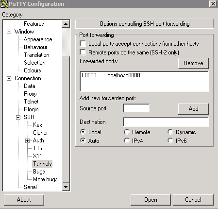
Next click the + SSH on the bottom left, and then click tunnels. You can now enter the port you want to access Jupyter on your local machine (for example 8000), and set the destination as localhost:8888 where 8888 is the number of the port that Jupyter notebook is running on. Now click the add button and the ports should appear in the Forwarded ports: section.
For the example of uWaterloo’s csclub, my Putty configuration screen looks like the following:
Finally you can hit open, and you will now both connect to the server via SSH and tunnel the desired ports. If no error shows up and you tunneled the port to 8000 (for example), you can simply navigate to localhost:8000 in our favourite web browser to connect to Jupyter notebook running on the server!
Using Jupyter notebook
Jupyter notebook will show all of the files and folders in the directory it is run from. We can now create a new notebook file by click new > python2 from the top right. This will open a notebook. We can now run python code in the cell or change the cell to markdown (by Cell > Cell Type > Markdown) and write notes and even put equations in by putting them between the $$ symbols. For example, to generate you can write the following
$$ y = x^2$$
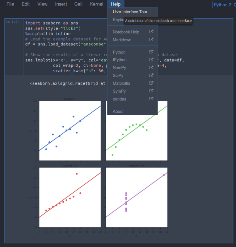
You can also download Jupyter Notebooks off the internet and open them in Jupyer. For now let us make a simple plot from the Anscombe’s quartet using the seaborn library. We can do this by just typing the following into the first cell
import seaborn as sns
sns.set(style="ticks")
%matplotlib inline
# Load the example dataset for Anscombe's quartet
df = sns.load_dataset("anscombe")

# Show the results of a linear regression within each dataset
sns.lmplot(x="x", y="y", col="dataset", hue="dataset", data=df,
           col_wrap=2, ci=None, palette="muted", size=4,
           scatter_kws={"s": 50, "alpha": 1})
Please note we use %matplotlib inline for the plots to appear inline in the notebook (instead of a pop-up). When using Jupyter Notebook, the easiest way to see a plot is in-line.
To get a quick tour of Jupyter notebook, you can go to Help > User Interface Tour as show below:
Once you have installed everything and Jupyter is running you can move onto to installing R and RStudio by following the Absolute Beginners Tutorial for Getting Started Doing Data Science using Servers.