Regression
Regression is fitting a line or curve to do numeric prediction or to do predicted causility analysis (in some cases).
Generalized linear models
Linear regression
Fit a line to a set of data, for example think Scatter plot of Grade vs. Hours of Study
| Hours of study | Grade |
|---|---|
| data1 | data1 |
| … | … |
Simple linear regressoin (with one feature (or attribute)):
Input:
| id | x | y | ŷ | y-ŷ |
|---|---|---|---|---|
| p1 | 1 | 2 | 1 | 1 |
| p2 | 1 | 1 | 1 | 0 |
| p3 | 3 | 2 | 3 | -1 |
Where x is a feature, y is the true output, ŷ is the predicted output and y-ŷ is called residual (observed - predicted)
Suppose we obtain in the following linear model:
y = x
Sum of the squares residuals (SSQ) =
Ordinary least squares (OLS) or linear least squares computes the least squares solution using a singular value decomposition of X. This means the algorithm attempts to minimize the sum of squares of residuals. If X is a matrix of size (n, p) this method has a cost of , assuming that . This means that for small number of features, the algorithm scales very well, but for a large number of features (p), it is more efficient (in terms of run time) to use a gradient descent approach after feature scaling. You can read more about the theory here and in more detail here
Other related metrics:
Mean Squared Error (MSE) =
Root Mean Squared Error (RMSE) =
In example:
SSQ =
MSE = 2/5
RMSE =
More complicated Example
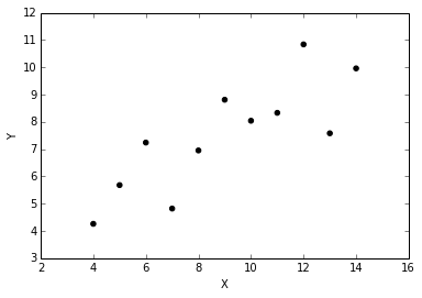
Now let’s take a look at one of the datasets from Anscombe’s quartet. The full analysis and code to generate the figures are outlined in the simple linear regression tutorial
| x | y | |
|---|---|---|
| 0 | 10 | 8.04 |
| 1 | 8 | 6.95 |
| 2 | 13 | 7.58 |
| 3 | 9 | 8.81 |
| 4 | 11 | 8.33 |
| 5 | 14 | 9.96 |
| 6 | 6 | 7.24 |
| 7 | 4 | 4.26 |
| 8 | 12 | 10.84 |
| 9 | 7 | 4.82 |
| 10 | 5 | 5.68 |
The scatter plot looks like:
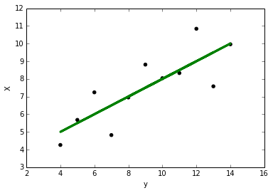
We can now use simple least squares linear regression to fit a line:
The residual (difference between y and y predicted (ŷ)) can then be calculated. The residuals looks like:
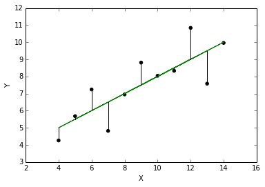
y - ŷ vs x can now be plotted:
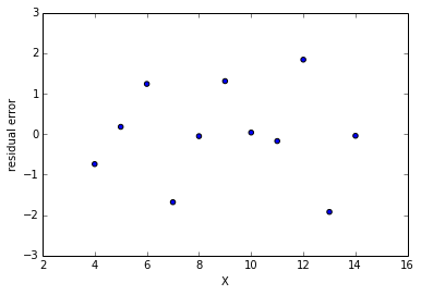
We can now plot the residual distribution:
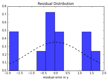
As seen the the histogram, the residual error should be (somewhat) normally distributed and centered around zero. This post explains why.
Vertical vs Horizontal vs Orthogonal Residuals

Usually we calculate the (vertical) residual, or the difference in the observed and predicted in the y. This is because “the use of the least squares method to calculate the best-fitting line through a two-dimensional scatter plot typically requires the user to assume that one of the variables depends on the other. (We caculate the difference in the y) However, in many cases the relationship between the two variables is more complex, and it is not valid to say that one variable is independent and the other is dependent. When analysing such data researchers should consider plotting the three regression lines that can be calculated for any two-dimensional scatter plot.
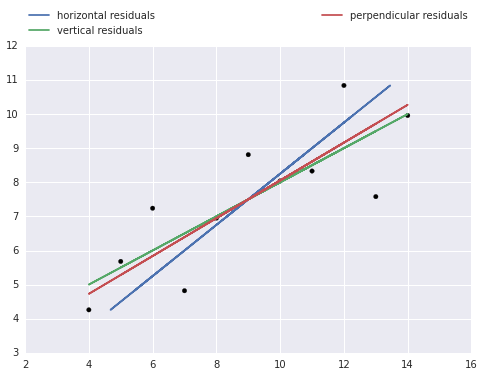
Plotting all three regression lines gives a fuller picture of the data, and comparing their slopes provides a simple graphical assessment of the correlation coefficient. Plotting the orthogonal regression line (red) provides additional information because it makes no assumptions about the dependence or independence of the variables; as such, it appears to more accurately describe the trend in the data compared to either of the ordinary least squares regression lines.” You can read the full paper here
Simple linear regression tutorial covers a complete example with all three types of regression lines.
- create residual plot for each feature and if x and y are indeed linearly related, the distribution of residuals should be normal and centered around zero
- if poor fit, consider applying a transform (such as log transform) or non-linear regression
- residual plot should not have any patterns (under/over estimation bias)
- residual plot is a great visualization of fit, but should be used in combination of other statiscal methods (see tutorial 2 and 3)
- After an initial model is created, it can be modified by doing a data transform, changing the features (called feature engineering) or model selection.
Data transforms
It linearizes the model so linear regression can be used on some non-linear relationships.
For example, if x is expoential compared to y apply log transform:
There are other methods for transforming variables to achieve linearity outlined [here](http://stattrek.com/regression/linear-transformation.aspx?Tutorial=AP:
| Method | Transformation(s) | Regression equation | Predicted value (ŷ) |
|---|---|---|---|
| Standard linear regression | None | ||
| Exponential model | Dependent variable = log(y) | ||
| Quadratic model | Dependent variable = sqrt(y) | ||
| Reciprocal model | Dependent variable = 1/y | ||
| Logarithmic model | Independent variable = log(x) | ||
| Power model | Dependent variable = log(y) | ||
| Independent variable = log(x) |
Transforming a data set to enhance linearity is a multi-step, trial-and-error process.
- Conduct a standard regression analysis on the raw data.
- Construct a residual plot.
- If the plot pattern is random, do not transform data.
- If the plot pattern is not random, continue.
- Compute the coefficient of determination (R2).
- Choose a transformation method (see above table).
- Transform the independent variable, dependent variable, or both.
- Conduct a regression analysis, using the transformed variables.
- Compute the coefficient of determination (R2), based on the transformed variables.
- If the tranformed R2 is greater than the raw-score R2, the transformation was successful. Congratulations!
- If not, try a different transformation method.
Generalized and Non-linear regression tutorial outlines an example of linear regression after a log transformation.
Feature Transformations
- Forward Selection
Try each variable one by one and find the one the lowest sum of squares error
- not used in practice
- Backward Selection (more practical than FS)
- Try with all the variables and remove the worse one (greedy algorithm) (bad variable = highest impact on SSQ)
- Shrinkage
- LASSO: uses matrix algebra to shrink coefficient to help with eliminating variables
The techniques are used in preparing data section and are outlined in the Scikit-learn documentation
Linear and Non-linear Regression using Generalized Linear Models
Piece-wise regression, polynomial regression, ridge regression, bayesian regression and many more generalized linear models are all valid methods of applying regression depending on the application. The Scikit Learn documentation has a very good outline and examples of many different techniques and when to use them. In addition the statsmodels library in python also provides an even more powerful implemention of regression with additional statistical properties as we saw in the tutorial.
Advanced Regression Techniques
In addition, we learn later in the course about classification methods which can also be used for regression. These include decision trees, nearest neighbour, support vector regression, isotonic regression.
For now, understand that these methods exist, and by applying the principles of model selection, evaluation and parameter tuning, you can identify which algorithm and method to use.
Multi-Regression
After regression with 1 single feature, the intuition can be extended to deal with multiple features called multi-regresion In simple linear regression, a criterion variable is predicted from one predictor variable. In multiple regression, the criterion is predicted by two or more variables. The basic idea is to find a linear combination of each of the features to predict the output. The problem is to find the values of and b in the equation shown below that give the best predictions. As in the case of simple linear regression, we define the best predictions as the predictions that minimize the squared errors of prediction.

Instead of a line for one features and an output, with more than one feature, the result is a plane. Tutorial 4 covers examples of multi-regression with real world data.